Model Optimization

Most deep learning models are made up of millions/billions of parameters. So, when we inference a model, we need to load all its parameter in the memory, this means big models cannot be loaded easily on a edge/embedded devices. So, this blog is focused on optimizing a model through different techniques and analyze its effect on inference time, model size, accuracy.

Model optimization is transforming machine/deep learning model such that it has:

1. Faster Inference Time

2. Reduction in network size (memory efficient)

We’re going to cover different topics, so buckle up

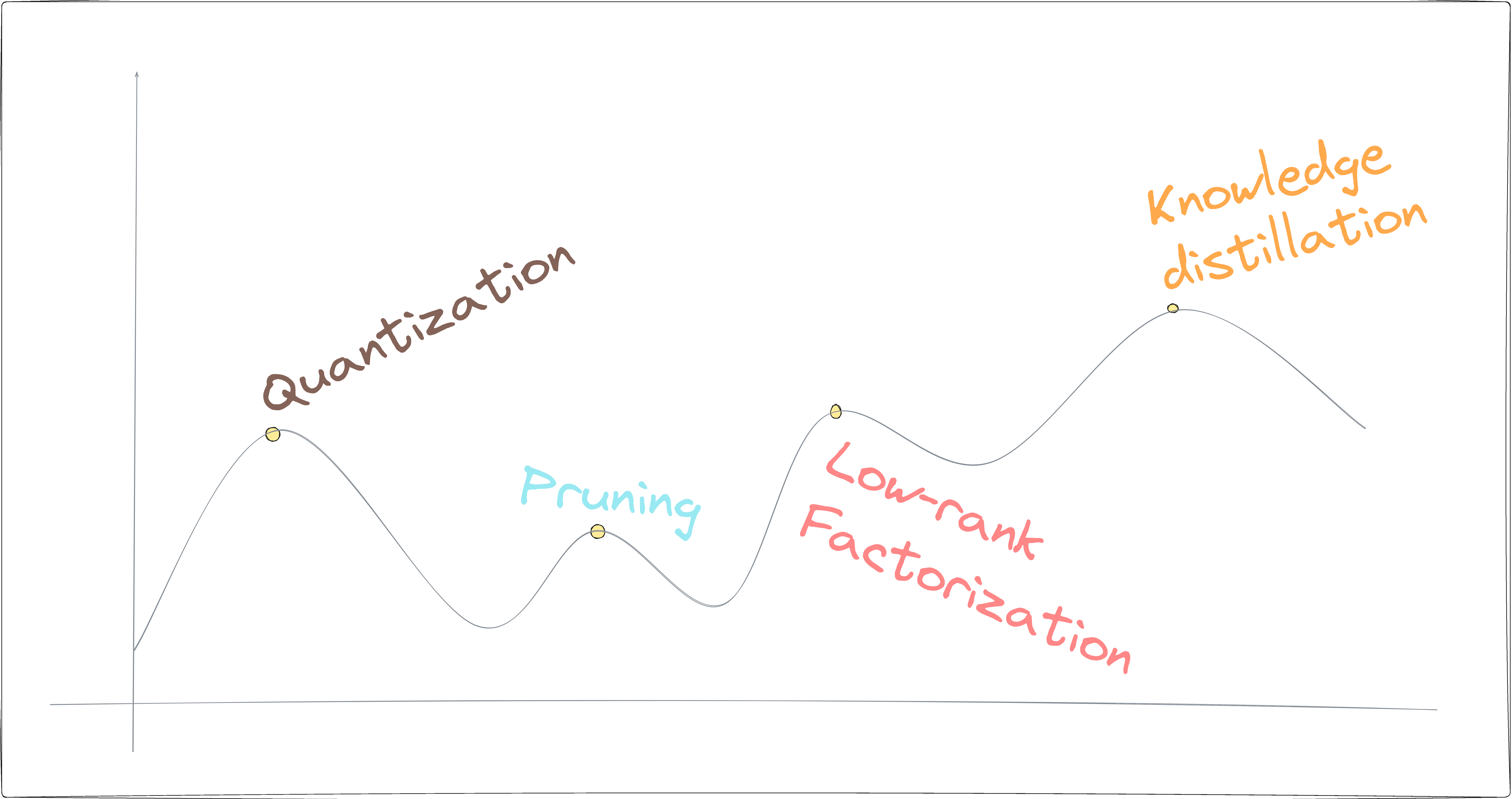
1. Quantization:
   Reducing number of bits used for model parameters

2. Network Pruning:
   Reducing the number of distinct weight values

3. Low-Rank Matrix Factorization:
   Factorizing model weights such that it reduces overall model parameters

4. Knowledge Distillation:
   Obtatining a smaller network by mimicking the prediction

We’ll mainly focus on optimizing pytorch model. But the gist we’ll be same for Tensorflow/caffe.,etc

1. Quantization

Quantization means converting/reducing the model parameters precision to lower bit precision typically 8-bit integers , without retraining the model.

Remapping from float32 to int8:

Calculation

To map the floating-point values to integer values, we need to calculate two key parameters:

1. Scale
   Step size between quantized values.

$$scale = \frac{max_{float} - min_{float}}{max_{int} - min_{int}}$$

For int8, $$min_{int} = -127$$ $$max_{int} = 127$$

2. Zero point
   Integer value that corresponds to the floating-point value of zero.
   $$zero_{point} = min_{int} - \frac{min_{float}}{scale}$$

Quantize the Float Values

Once the scale and zero point are determined, each floating-point value 𝑥 can be quantized to an integer value 𝑞 using:

$$q = \text{round} \left( \frac{x}{scale} + zero_{point} \right)$$

De-Quantize the Float Values

To convert back from quantized values 𝑞 to floating-point values 𝑥, we use:

𝑥 = scale⋅(𝑞 − zero_point)

$$x = scale \cdot (q - zero_{point})$$

Pytorch Availability

1. Half Precision

Half precision refers to performing computations using 16-bit floating point numbers(half precision) instead of standard 32-bit floating point numbers(single precision) to accelerate inference process.

Using half precision, the memory requirements and computational cost of the inference process can be reduced, leading to faster inference time.

Blockers:
i. As of now, Half-Precision is not supported for CPU. Operations for conv_layer, stft, etc doesn’t support operations in float-16 on cpu.

2. Post Training Dyanmic Quantization

In Dynamic Quantization, the quantization on model weights are quantized ahead of time while quantization on activations occurs dynamically during runtime.
During inference, the activation’s are collected for input and are analyzed to determine their dynamic range. Once the dynamic range is known, quantization parameters such as scale and zero-point are calculated to map the floating point activation to lower precision.

Implementation

import torch
model = …  #pytorch model
quantized_model = torch.ao.quantization.quantize_dynamic(model, qconfig_spec={torch.nn.Linear}, dtype=torch.qint8)
output = quantized_model(input) #infer on quantized model

- Supported Layers:

1. nn.Linear
2. nn.LSTM / nn.GRU / nn.RNN
3. nn.Embedding

3. Post Trianing Static Quantization

Scales and zero points for all the activation tensors are pre-computed using some representative unlabeled data.

Given a floating point Dense Neural Network(DNN), we would just have to run the DNN using some representative unlabeled data, then collect the distribution statistics(scale point and zero point) for all the activation layers.
This quantization minimizes the model performance degradation by estimating the range of numbers that the model interacts with using a representative dataset.

Blockers:

• Conv packing expects numerical padding as an input.

• The “same“ padding computation is not implemented internally in the quantized convolutional layer.

Implementation

1. First, we need to insert torch.quantization.QuantStub and torch.quantization.DeQuantStub operations before and after the network for the necessary tensor conversions.
   Consider we have simple Pytorch model with a simple linear layer Linear(10, 20)

import torch
class OriginalModel(torch.nn.Module):
    def __init__(self):
        super(M, self).__init__()
        # QuantStub converts the incoming floating point tensors into a quantized tensor
        self.quant = torch.ao.quantization.QuantStub()
        self.linear = torch.nn.Linear(10, 20)
        # DeQuantStub converts the quantized tensor into a floating point tensors
        self.dequant = torch.ao.quantization.DeQuantStub()
    
    def forward(self, x):
    # using QuantStub and DeQuantStub ops, we indicate the region for quantization in a model
        x = self.quant(x)
        x = self.linear(x) # original model
        x = self.dequant(x)
        return x

2. Model is instanstiated and trained

# model is instantiated and trained
model_fp32 = OriginalModel()

# Prepare the model for static quantization
model_fp32.eval()
model_fp32.qconfig = torch.ao.quantization.get_default_qconfig('fbgemm')
model_fp32_prepared = torch.ao.quantization.prepare(model_fp32)

# Determine the best quantization settings by calibrating the model on a representative dataset.
calibration_dataset = torch.utils.data.Dataset...
model_fp32_prepared.eval()
for data, label in calibration_dataset:
    model_fp32_prepared(data)

if the target environment is mobile device, we must pass in ‘qnnpack’ to the get_default_qconfig function and for server inference, ‘fbgemm’ or ‘x86’.

3. Convert calibrated model to a quantized model

model_int8 = torch.ao.quantization.convert(model_fp32_prepared)

2. Pruning

Pruning is a technique of identifying and removing unimportant or redundant parameters, such as weights and neurons, from the network. Removing unimportant parameters from a trained neural network model helps to reduce its size and computational complexity Here we’ll be doing Post-training pruning which involves pruning the trained model. In general we’ve two types of pruning.

1. Global Unstructured Pruning

• It involves removing individual model weight parameters based on their magnitude or importance.
• It prunes the entire network at once, considering the importance of each parameter across the entire model.
• Even if weights are pruned to zero in global unstructured pruning, the underlying matrix operations is same to that of the dense original network. So, basically it will have same inference time. One major limitation of DL framework today is the lack of sparse operation which can be benefited in case like this.

2. Local Structured Pruning

• It involves removing entire structured groups of weights, such as channels or neurons, based on their importance or contribution to the model’s performance.
• It prunes at the level of individual neurons, connections, or weights within a layer of the neural network.
• This method guarantees that connections to a neuron in a linear layer or channels in a convolutional layer will be zeroed out. This means that if a channel or neuron is completely unimportant, it can be safely removed without affecting the model’s performance. So we’ll be focusing more on the Local Structured Pruning

Linear Layer

Fig., (a) Dense Network (b) Pruned Network (dotted lines represent pruned neurons and connections) (c) Network in which the pruned neurons are actually removed from the architecture.

Considering a single Linear Layer

linear_layer = nn.Linear(in_features=10, out_features=100)

The weight for this linear layer will be:

torch.Size(100, 10)
- This means that each of the 100 output neurons has a connection to each of the 10 input neurons, resulting in a weight matrix of 100 rows and 10 columns.

Now After we apply Local Structured Pruning, it guarantee that some neruons will be zeroed out, so we can physically remove those connections to that particular neurons. Following are the steps:

1. Identify Redundant Neurons: Determine which neurons (rows in the weight matrix) are redundant. These neurons will have weights and biases that can be set to zero.

2. Remove connections and replace weights with new Linear Layer: Physically remove the connections associated with these redundant neurons. This means removing the corresponding rows in the weight matrix and the associated biases. and then create a new smaller linear layer that has reduced weight and biases from above.

3. Preserve Output Shape:
   To maintain the original output shape, zero-padding is added back to the output tensor at the positions corresponding to the removed neurons. This ensures that the output shape of the pruned layer matches the original layer.

What if we have subsequent linear layers? When dealing with subsequent layers, the input to these layers will also be affected by the pruning of the previous layer. The steps are as follows:

1. Identify Pruned Neurons in Previous Layer:
   Identify which neurons were pruned in the previous layer.

2. Adjust Weight Matrix of the Next Layer:
   Modify the weight matrix of the subsequent linear layer to account for the removed input connections. Essentially, this means removing the corresponding columns in the weight matrix of the next layer.

3. Create Reduced Linear Layer:
   Similar to the previous layer, create a new linear layer with the reduced number of input features.

Convolution Layer

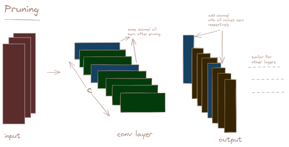
In case of convolution layer as well, the idea is same, we identify the redundant channel and perform convolution without considering those redundant channels and later add zeroed channel on those previous zeroed index channels.

3. Low Rank Matrix Factorization

Matrix Factorization is decomposing matrices into smaller sub-matrices which serve as approximation of the original matrices while having fewer parameters.

The Singular Valued Decomposition(SVD) lets us decompose any matrix A with n rows and m columns:

where, r are singular values and if we take first k largest singular values and set other to zero , we’ll get an approximation of A.

Let’s see how matrix factorization helps with the model compression or faster inference.

Example:

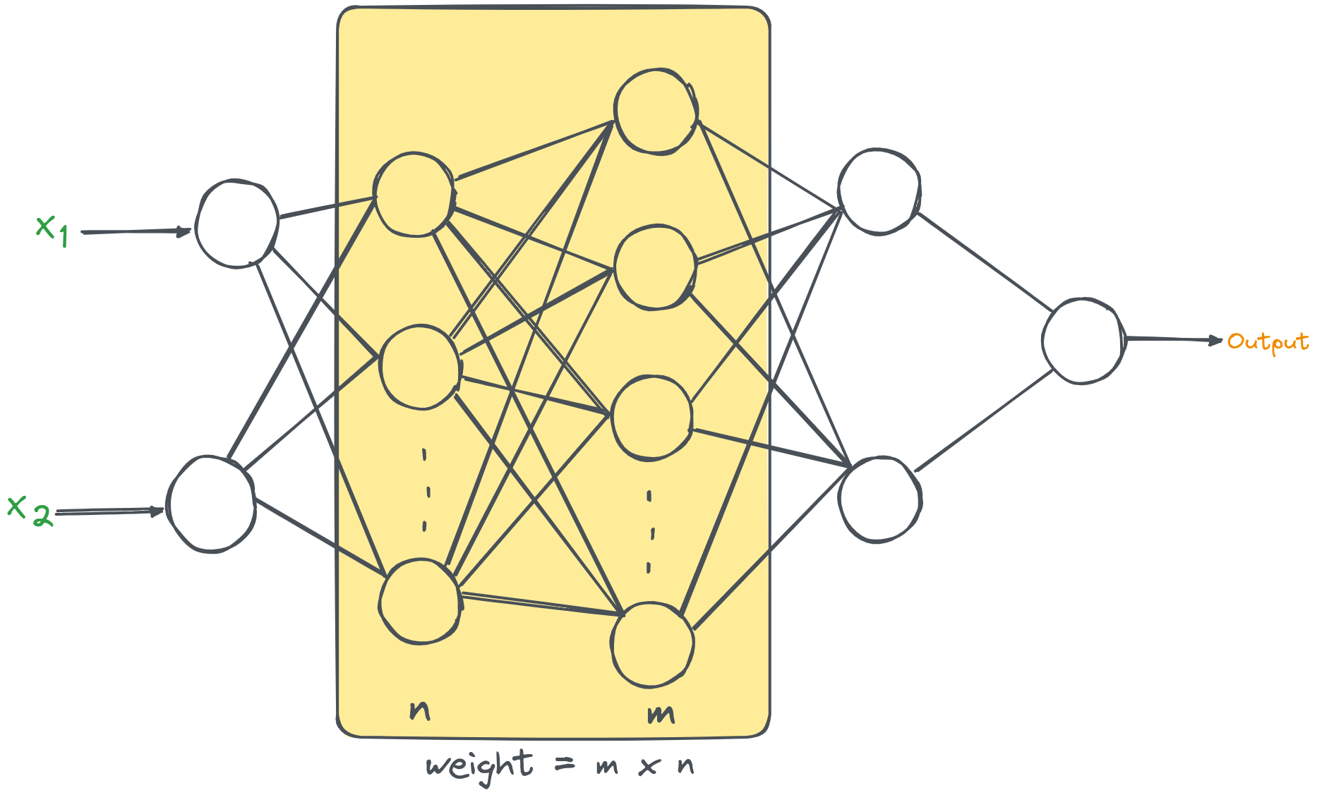
For 2nd and 3rd layer, If we consider n=1000, and m=500,

Without low-rank matrix factorization:

Number of parameters in W = m * n = 500,000 parameters

With low-rank matrix factorization:

W is decompose into lower-rank matrices U and V.

Number of parameters in U = m × k = 500 × 50 = 25,000 parameters.

Number of parameters in V = k × n = 50 × 1000 = 50,000 parameters.

Total number of parameters = 25,000 + 50,000 = 75,000 parameters.

    Low rank approximation decreases parameters. from nm to k(n+m).

Problem

We are given a matrix W and want to find a low rank matrix that produces the lowest approximation error to W.

• Find rank for each layer, but if we find rank ahead of time to use in each layer. Then we can write weight matrix at each layer as UkVkT and optimize the network as usual over all Uk , Vk matrices.

Now, let’s explore how we can apply this low rank decomposition on the fully-connected layers and convolution layers

Post Training Weight/Kernel Decomposition

1. SVD on a Fullly Connected Layer

A fully connected layer essentially does matrix multiplication of its input by a weight matrix, and then adds a bias b: Wx + b

We can take the SVD of weight matrix, and keep only the first k singular values.

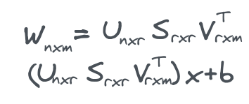
Instead of a single fully connected layer, we implement it as two smaller fully connected layers:

• The first one will have a shape of mxr, with no bias, and its weights will be taken from SVT.

• The second one will have a shape of rxn, with bias equal to b, and its weights will be taken from .

The total number of weights dropped from nxm to r(n+m).

2. Tensor Decomposition on Convolution Layers

The idea is similar to above. We use the weight of convolution layer and apply some decomposition on the weight matrix and the decomposed weight matrix is represented by some smaller size convolution layer which performs depth-wise and point-wise operations.

There are different algorithm for it:

1. CP Decomposition
2. Tucker Decomposition

4. Knowledge Distillation

It is a technique where we train a smaller, more efficient student model to mimic the behavior of a larger, more complex teacher model. The central idea is to transfer the ‘knowledge ’ embedded within the cumbersome teacher model to the compact student model. Due to this simpler architecture, KD helps for faster inference and deployment on devices with limited resources.

Components of Knowledge Distillation

1. Knowledge

The valuable information embedded within a complex, well-trained deep learning model (the teacher) that we aim to transfer to a smaller model (the student). Knowledge can be categorized into:

• Response-Based Knowledge:
  Information derived from the final output predictions of the teacher model. This typically involves soft probabilities (in classification tasks) or continuous values (in regression tasks).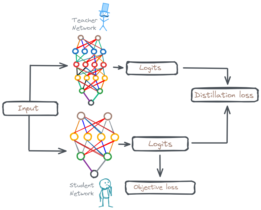

• Feature-Based Knowledge:
  Knowledge captured in the intermediate feature representations (outputs of hidden layers) of the teacher network. This encodes higher-level abstractions learned by the teacher.

• Relationship-Based Knowledge:
  Knowledge about how different data samples interact with each other, or how different parts of the model interact.

2. Distillation

The mechanism by which knowledge is transferred from the teacher to the student. This involves:

• Loss Functions:
  Loss functions tailored to the type of knowledge being transferred. Common choices include:

  • Kullback-Leibler (KL) Divergence for response-based knowledge (often used with probability distributions).

  • Mean Squared Error (MSE) for response-based (continuous outputs) and feature-based knowledge.

  • Perceptual losses and Gram matrix losses for feature-based knowledge.

Training Scheme

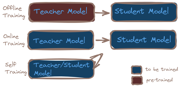
• Offline Distillation:

  • Teacher Training:
    Utilize a larger, pre-trained model

  • Student Training:

    • Feed data to both the teacher and the student models.

    • Calculate the distillation loss based on the difference between the teacher’s soft predictions and the student’s predictions.

    • Calculate the objective loss function based on the student’s predicted and the ground truth.

    • Combine the distillation loss and the additional loss, to form the overall training loss.

• Online Distillation:
  Knowledge is transferred by employing both Teacher and student training.

• Self-Distillation:
  The same model serves as both teacher and student (after some initial training).

3. Teacher-Student Architecture

The relationship between the complexity and capacity of the teacher and the student models:

• Teacher Model:
  Usually a large, pre-trained model with superior performance. This model could be a complex ensemble or a model trained with extensive compute resources.

• Student Model:
  A smaller, more computationally efficient model. It is designed to be deployable in scenarios with limited resources (e.g., mobile devices, embedded systems) while still maintaining good performance.

References:

• Pruning + Information Flow Knowledge Distillation
• Comprehensive Guide to Pruning